MetroSCREEN(RNA-seq)

For bulk RNA-seq data, MetroSCREEN calculates the MetaModule score for each sample and constructs a MetaRegulon for each dysregulated MetaModule, offering insights into the mechanisms of metabolic regulation. Additionally, MetroSCREEN identifies the sources of the MetaRegulons. Given that several samples may not be suitable for inferring causation between MetaModules and MetaRegulons, directions for bulk RNA-seq data are not provided.

To demonstrate how the MetaModule and MetaRegulon functions of MetroSCREEN are used with bulk RNA-seq data, we have provided a demo dataset available here.

Step 1 MetaModule analysis

1. Prepare the metabolic information

We utilized the metabolic reactions and corresponding information provided by Recon3D. Since some of this information is duplicated, we have provided a simplified version. Users can download it from here. Alternatively, users can manually create and use gene sets of interest. We recommend that both the treatment and control groups contain at least three sets of data.

library(MetroSCREEN)

## Metabolic reactions and detaild description for them
MM=readRDS("./ref/MM.nodup.rds")
MM.meta=readRDS("./ref/MM.meta.rds") %>% as.data.frame()
rownames(MM.meta)=MM.meta$ID

MM[1:2]
# $`HMR-0154`
# 'ACOT7''ACOT2''ACOT9''BAAT''ACOT4''ACOT1''ACOT6'
# $`HMR-0189`
# 'ACOT7''ACOT2''BAAT''ACOT4''ACOT1''ACOT6'

MM.meta[1:3,]
#    ID      NAME    EQUATION        EC-NUMBER       GENE ASSOCIATION        LOWER BOUND     UPPER BOUND     OBJECTIVE       COMPARTMENT     MIRIAM  SUBSYSTEM       REPLACEMENT ID  NOTE    REFERENCE       CONFIDENCE SCORE
# <lgl>      <chr>   <chr>   <chr>   <chr>   <chr>   <lgl>   <lgl>   <lgl>   <lgl>   <chr>   <chr>   <lgl>   <lgl>   <chr>   <dbl>
# HMR-0154   NA      HMR-0154        NA      H2O[c] + propanoyl-CoA[c] => CoA[c] + H+[c] + propanoate[c]             3.1.2.2 ENSG00000097021 or ENSG00000119673 or ENSG00000123130 or ENSG00000136881 or ENSG00000177465 or ENSG00000184227 or ENSG00000205669       NA      NA      NA      NA      sbo/SBO:0000176 Acyl-CoA hydrolysis     NA      NA      PMID:11013297;PMID:11013297     0
# HMR-0189   NA      HMR-0189        NA      H2O[c] + lauroyl-CoA[c] => CoA[c] + H+[c] + lauric acid[c]              3.1.2.2 ENSG00000097021 or ENSG00000119673 or ENSG00000136881 or ENSG00000177465 or ENSG00000184227 or ENSG00000205669                          NA      NA      NA      NA      sbo/SBO:0000176 Acyl-CoA hydrolysis     NA      NA      NA                              0
# HMR-0193   NA      HMR-0193        NA      H2O[c] + tridecanoyl-CoA[c] => CoA[c] + H+[c] + tridecylic acid[c]      3.1.2.2 ENSG00000097021 or ENSG00000119673 or ENSG00000136881 or ENSG00000177465 or ENSG00000184227 or ENSG00000205669                          NA      NA      NA      NA      sbo/SBO:0000176 Acyl-CoA hydrolysis     NA      NA      NA                              0

2. Calculate the MetaModule score

In this section, MetroSCREEN calculates the MetaModule score for each sample using cal_MetaModule function. To identify differentially enriched MetaModules for each group in the experimental design, we use the FindAllMarkers_MetaModule function from MetroSCREEN. This function is similar to the FindAllMarkers function in Seurat, allowing users to employ similar parameters. The results from cal_MetaModule will be stored in the ./CCLE/ folder.

expression<-readRDS('./CCLE/ccle.rds')
## Calculate the MetaModule score
cal_MetaModule(expression,MM,'./CCLE/','ccle_gsva')
ccle.gsva=readRDS('./CCLE/ccle_gsva.rds')

3. MetaModule score exploration

## Read the sample information object for each sample
sample_info<-readRDS('./CCLE/ccle_meta.rds')

head(sample_info)

# NCIH2106Non-Small Cell Lung CancerUPCISCC040Head and Neck Squamous Cell CarcinomaUPCISCC074Head and Neck Squamous Cell CarcinomaUPCISCC200Head and Neck Squamous Cell CarcinomaNCIH1155Non-Small Cell Lung CancerNCIH1385Non-Small Cell Lung Cancer
# Levels:
# 'Head and Neck Squamous Cell Carcinoma''Non-Small Cell Lung Cancer'

## Find the differentially enriched MetaModule for each group
MetaModule.markers=FindAllMarkers_MetaModule(ccle.gsva,sample_info,'bulk')
MetaModule.markers$metabolic_type=MM.meta[MetaModule.markers$gene,'SUBSYSTEM']
MetaModule.markers$reaction=MM.meta[MetaModule.markers$gene,'EQUATION']

head(MetaModule.markers)

# p_val      avg_log2FC      pct.1   pct.2   p_val_adj       cluster gene    metabolic_type  reaction
# <dbl>      <dbl>   <dbl>   <dbl>   <dbl>   <fct>   <chr>   <chr>   <chr>
# HMR-4843   3.755633e-05    2.730885        1       0       0.06418377      Head and Neck Squamous Cell Carcinoma   HMR-4843        Transport reactions     GDP[c] + GTP[m] <=> GDP[m] + GTP[c]
# HMR-1969   9.059557e-05    2.891705        1       0       0.15482783      Head and Neck Squamous Cell Carcinoma   HMR-1969        Androgen metabolism     dehydroepiandrosterone[c] + PAPS[c] => dehydroepiandrosterone sulfate[c] + H+[c] + PAP[c]


saveRDS(MetaModule.markers,'./CCLE/ccle_gsva_markers.rds')

4. Visualization

Here, we give two examples for the following analysis.

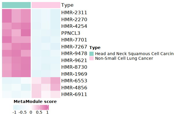
## Show the top 10 most enriched MetaModule for each group
top10<- MetaModule.markers %>%
   group_by(cluster) %>%
   arrange(desc(avg_log2FC), .by_group = TRUE) %>%
   slice_head(n = 10) %>%
   ungroup()

doheatmap_feature(ccle.gsva,sample_info,top10$gene,6,4,cols=c('Head and Neck Squamous Cell Carcinoma'='#8DD3C7','Non-Small Cell Lung Cancer'='#FCCDE5'))

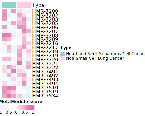
If users are interested in a specific pathway and wish to identify the detailed reactions that differentiate various groups, they can exclusively configure the pathways.

## Here we give an example with Chondroitin / heparan sulfate biosynthesis pathway
doheatmap_feature(ccle.gsva,sample_info,MM.meta[MM.meta$SUBSYSTEM=='Chondroitin / heparan sulfate biosynthesis','ID'],5,4,
              cols=c('Head and Neck Squamous Cell Carcinoma'='#8DD3C7','Non-Small Cell Lung Cancer'='#FCCDE5'))

Step 2 MetaRegulon analysis

MetroSCREEN systematically considers the combined effects of intrinsic cellular drivers and extrinsic environmental factors on metabolic regulation.

1. Prepare the essential files

To find the marker genes for each group, which is essential for calculating MetaRegulon activity, use the following approach.

## Read sample expression and group information
expression<-readRDS('./CCLE/ccle.rds')
sample_info<-readRDS('./CCLE/ccle_meta.rds')

## Considering the TPM format for the expression data, the limma package was utilized. If the expression is raw count, please use the DESeq2 package
group_list <- factor(c(rep("control",1), rep("treat",3),rep("control",2)))
design <- model.matrix(~sample_info)
colnames(design) <- levels(group_list)
rownames(design) <- colnames(expression)

fit <- lmFit(expression, design)
fit <- eBayes(fit)
DE_genes <- topTable(fit, coef = 2,p.value = 0.05, lfc = log2(1.5), number = Inf,sort.by="logFC")

DE_genes$cluster=ifelse(DE_genes$logFC>0,'Head and Neck Squamous Cell Carcinoma','Non-Small Cell Lung Cancer')
DE_genes$gene=rownames(DE_genes)
DE_genes=DE_genes[order(abs(DE_genes$logFC),decreasing = TRUE),]
saveRDS(DE_genes,'./CCLE/ccle_gene_markers.rds')

Prepare the Lisa results for each group, as these are essential for calculating MetaRegulon TR activity. Users can learn more about Lisa here.

for (i in unique(DE_genes$cluster)){
   df=DE_genes[DE_genes$cluster==i,]
   if (nrow(df)>500){
      genes=df[,'gene'][1:500]
   } else{ß
      genes=df[,'gene']
   }

   write.table(genes,paste0('./CCLE/lisa/',i,':marker.txt'),
            sep='\t',
            quote=F,
         row.names=FALSE,
         col.names=FALSE)
}

## Run this under Lisa's guidance
lisa multi hg38 ./CCLE/lisa/*.txt -b 501 -o ./CCLE/lisa/

2. Calculate the MetaRegulon score

The MetaRegulon for a MetaModule can be inferred using the cal_MetaRegulon function. MetroSCREEN employs a four-step strategy to deduce the MetaRegulon: Inferring the activity of the MetaRegulon is the first step.

Correlating MetaRegulon activity with gene expression within the MetaModule constitutes the second step. We consider the highest correlation value among the genes in a MetaModule as representative of the interaction between the MetaRegulon and the MetaModule.

Using a multi-objective optimization method to determine the most likely MetaRegulon to control the MetaModule is the third step.

Inferring causation between the MetaModule and MetaRegulon using a PC-based method is the fourth step.

## Users can replace the metabolic reaction with one they are interested in
MM=readRDS("./ref/MM.nodup.rds")
MM.meta=readRDS("./ref/MM.meta.rds") %>%
   as.data.frame()
rownames(MM.meta)=MM.meta$ID

metacell.seurat <- CreateSeuratObject(counts = expression, project = "bulk", min.cells = 0, min.features = 0)
metacell.seurat@meta.data$sample=as.factor(c(rep("Non-Small Cell Lung Cancer",1), rep("Head and Neck Squamous Cell Carcinoma",3),rep("Non-Small Cell Lung Cancer",2)))
MetaModule.markers<-readRDS('./CCLE/ccle_gene_markers.rds')

## set the parameters
object=metacell.seurat
feature='sample'
state='Head and Neck Squamous Cell Carcinoma'
## Users can use the differentially enriched MetaModule
# interested_MM=MetaModule.markers[MetaModule.markers$cluster=='COL11A1+ CAF','gene']
interested_MM=c('HMR-7519','HMR-7510')
MM_list=MM
markers=DE_genes
lisa_file='./CCLE/lisa/Head and Neck Squamous Cell Carcinoma:marker.txt.lisa.tsv'
ligand_target_matrix='./ref/ligand_target_matrix.rds'
lr_network='./ref/lr_network.rds'
sample_tech='bulk'
output_path='./CCLE/'
RP_path='./ref/RP_score.rds'
file_name='HNSC'

Calculate the MetaRegulon score

cal_MetaRegulon(object,feature,state,interested_MM,MM_list,markers,lisa_file,ligand_target_matrix,lr_network,sample_tech,output_path,RP_path,file_name)

The results of the cal_MetaRegulon function will be stored in the ./CCLE/HNSC/ floder, and the detailed information is shown below.

File | Description
{file_name}.rds	The expression matrix of the state.
{file_name}:lr_activity.rds	The ligands activity for each sample.
{file_name}:tr_activity.rds	The transcriptional regulators activity for each sample.
{file_name}:gg_activity_cor.rds	The correlation of intrinsic signaling components activity with MetaModule.
{file_name}:tr_activity_cor.rds	The correlation of intrinsic transcriptional regulators activity with MetaModule.
{file_name}:lr_activity_cor.rds	The correlation of extrinsic ligands activity with MetaModule.
./MetaRegulon/{file_name}:*.txt	The MetaRegulon results.

It should be noted that since there is no interaction between individual samples, the ligands calculated in bulk RNA-seq data are mainly the result of autocrine signaling.

3. Downstream analysis

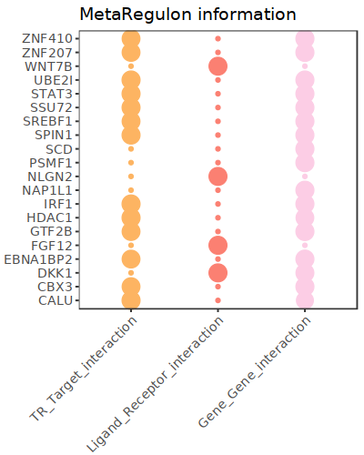
Resources of MetaRegulon.

hmr_7519<-read.csv(paste0(output_path,file_name,'/MetaRegulon/',file_name,':HMR-7519.txt'),row.names = 1)
head(hmr_7519,2)
# TR_Target_interaction      Ligand_Receptor_interaction     Gene_Gene_interaction   ag_score        .level  Final_score     gene    rank    resource
# <dbl>      <dbl>   <dbl>   <dbl>   <int>   <dbl>   <chr>   <int>   <chr>
# CALU       0.9995743       0.000000        0.8508204       0.003328891     1       0.003328891     CALU    1       intrinsic
# FGF12      0.0000000       0.996856        0.0000000       0.003328891     1       0.003328891     FGF12   2       extrinsic
df_use=melt(hmr_7519[1:20,c(1:3,7)])

width=4
height=5
options(repr.plot.width =width, repr.plot.height = height,repr.plot.res = 100)
ggplot(df_use, aes(x = variable, y = gene)) +
   geom_point(aes(color = variable, size = value)) +
   scale_color_manual(values = c("TR_Target_interaction" = "#FDB462", "Ligand_Receptor_interaction" = "#FB8072",'Gene_Gene_interaction'='#FCCDE5')) +
   theme_bw() +
   theme(
      panel.grid.major = element_blank(),
      panel.grid.minor = element_blank(),
      axis.text.x = element_text(angle = 45, hjust = 1),
      legend.position = "none"
   ) +
   theme(axis.title = element_text(size = 10), axis.text = element_text(size = 10),
         legend.text = element_text(size = 10), legend.title = element_text(size = 10))+
   labs(x = NULL, y = NULL, title = "MetaRegulon information")

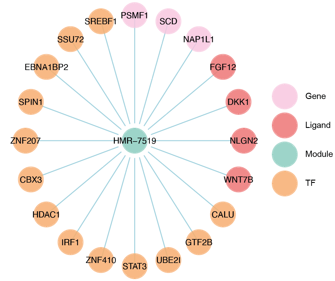
Build the network.

hmr_7519<-read.csv(paste0(output_path,file_name,'/MetaRegulon/',file_name,':HMR-7519.txt'),row.names = 1)
df_use=hmr_7519[1:20,]
network=data.frame(from=rownames(df_use),to='HMR-7519',#label=ifelse(df_use$direction=='regulator','1','2'),
                  color=ifelse(df_use$gene %in% df_use[df_use$Ligand_Receptor_interaction>0,'gene'],'Ligand',
                              ifelse(df_use$gene %in% df_use[df_use$TR_Target_interaction>0,'gene'],'TF','Gene')))
node=data.frame(unique(c(network$from,network$to)))
node$class=ifelse(node[,1] %in% 'HMR-7519','Module',
                  ifelse(node[,1] %in% df_use[df_use$Ligand_Receptor_interaction>0,'gene'],'Ligand',
                     ifelse(node[,1] %in% df_use[df_use$TR_Target_interaction>0,'gene'],'TF','Gene')))
colnames(node)=c('gene','class')
g <- graph_from_data_frame(d = network, vertices =node, directed = FALSE)
layout <- create_layout(g, layout = 'circle')

## Modify the layout
n=nrow(layout[layout$class %in% c('Ligand','TF'),c('x','y')])
theta <- seq(0,2*pi, length.out = 21)
coords <- data.frame(
x = sin(theta) ,
y =  cos(theta) )
layout[layout$class=='Gene',c('x','y')]=coords[1:3,]
layout[layout$class=='Ligand',c('x','y')]=coords[4:7,]
layout[layout$class=='TF',c('x','y')]=coords[8:20,]
layout[layout$class=='Module','x']=0
layout[layout$class=='Module','y']=0

Draw the network.

width=5.5
height=5
options(repr.plot.width =width, repr.plot.height = height,repr.plot.res = 100)
output_name='HMR-7519.pdf'

graph_g<-ggraph(layout)+   #kk
   geom_edge_link(color='lightblue',arrow = arrow(length = unit(0, 'mm')),end_cap = circle(8, 'mm'))+
   geom_node_point(aes(color=class),size = 15,alpha=0.8)+
   geom_node_text(aes(label = name),size=4) +
   scale_color_manual(values = c('Ligand'="#FB8072",'TF'="#FDB462",'Gene'='#FCCDE5','Module'='#8DD3C7')) +
   scale_edge_width(range=c(0.5,1.5))+
   theme(text = element_text(size=8))+
   theme_void()
print(graph_g)
pdf(paste0(output_path,output_name),width=width,height=height)
   print(graph_g)
dev.off()