MetroSCREEN(scRNA-seq)

For single-cell data, MetroSCREEN calculates the MetaModule score for each cell and then builds a MetaRegulon for the dysregulated MetaModule, which provides insights into the mechanisms of metabolic regulation. Besides, MetroSCREEN delineates the direction and source of the MetaRegulon for the MetaModule.

To demonstrate how the MetaModule and MetaRegulon functions of MetroSCREEN are used with scRNA-seq data, we have provided a demo dataset available here.

Step 1 Prepare the Metacell (Optional)

If users wish to achieve better results and save time, MetroSCREEN offers a Metacell strategy using the make_Metacell function to mitigate the impact of technical noise and increase gene coverage. More detailed information about this strategy can be found in TabulaTIME. The number of cells in a Metacell depends on the total cell count. If the total exceeds 3,000, the recommended number of cells per Metacell is 30. For smaller cell populations, users can set a lower number of cells per Metacell, but it should not be less than 10.

library(MetroSCREEN)

Fibro.seurat <- readRDS('./scRNA/fibro_new.rds')
options(repr.plot.width = 7, repr.plot.height = 5,repr.plot.res = 100)
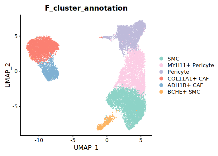
DimPlot(Fibro.seurat, reduction = "umap",group.by='F_cluster_annotation',cols=c('SMC'='#8DD3C7','MYH11+ Pericyte'='#FCCDE5','Pericyte'='#BEBADA','COL11A1+ CAF'='#FB8072','ADH1B+ CAF'='#80B1D3','BCHE+ SMC'='#FDB462'))

## Set the split with the cell subtypes information
Fibro.seurat$split=paste0(Fibro.seurat$F_cluster_annotation)

## Construct the Metacell
make_Metacell(Fibro.seurat,'split',10,'./scRNA/','fibro_new_Metacell')

## Metacell object can be read
Metacell<-readRDS('./scRNA/fibro_new_Metacell.rds')

## The rows of the Metacell are the genes, while the columns of the Metacell are the cell subtypes information.
Metacell[1:3,1:6]

# COL11A1+ CAF|2|1   COL11A1+ CAF|2|2        COL11A1+ CAF|2|3        COL11A1+ CAF|2|4        COL11A1+ CAF|2|5        COL11A1+ CAF|2|6
# A1BG       0.000000        0.000000        0.000000        0.000000        0.0000000       0.000000
# A1BG-AS1   0.000000        0.000000        0.000000        0.000000        0.4486995       0.000000
# A2M        1.658391        1.232226        2.295417        3.266894        2.6936025       3.799514

The results of make_Metacell will be stored in the ./scRNA/ floder, and the detailed information are shown as below.

File	Description
./scRNA/	The directory stores make_Metacell output files.
{outprefix}.rds	The Metacell expression matrix.
{outprefix}_info.rds	The detailed cell information in a Metacell.

After obtaining the Metacell object, users can analyze the Metacells expression data in a similar way as with single-cell expression data.

## Create Seurat object for Metacell/cell expression matrix
Metacell.seurat <- CreateSeuratObject(counts = Metacell, project = "Metacell", min.cells = 0, min.features = 0)

## Normalize data
Metacell.seurat <- NormalizeData(Metacell.seurat)

## Find variable features
Metacell.seurat <- FindVariableFeatures(Metacell.seurat, selection.method = "vst", nfeatures = 2000)

Metacell.seurat <- ScaleData(Metacell.seurat)
## Set the cell subtypes information for seurat object
Metacell.seurat@meta.data$cell_type=sapply(strsplit(rownames(Metacell.seurat@meta.data),"[|]"),
                             function(x) x[1])
Metacell.seurat <- RunPCA(Metacell.seurat)
Metacell.seurat <- RunUMAP(Metacell.seurat, dims = 1:10)
Metacell.seurat <- FindNeighbors(Metacell.seurat, dims = 1:10)
Metacell.seurat <- FindClusters(Metacell.seurat, resolution = 0.6)
options(repr.plot.width = 6, repr.plot.height = 5,repr.plot.res = 100)

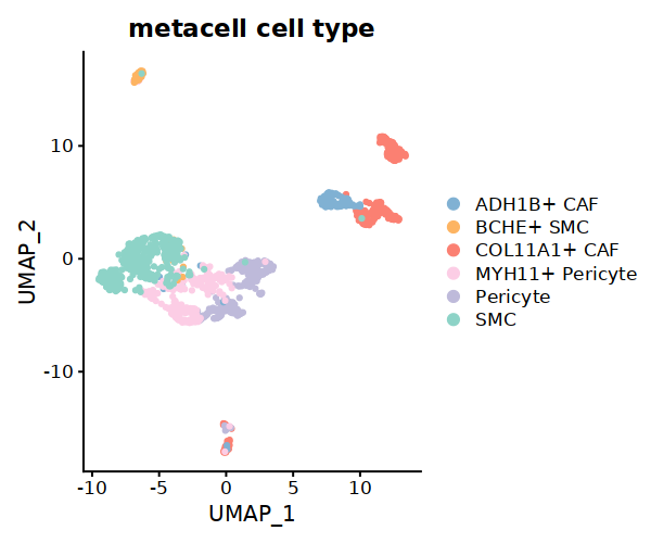
DimPlot(Metacell.seurat, reduction = "umap",group.by='cell_type',cols=c('SMC'='#8DD3C7','MYH11+ Pericyte'='#FCCDE5','Pericyte'='#BEBADA','COL11A1+ CAF'='#FB8072','ADH1B+ CAF'='#80B1D3','BCHE+ SMC'='#FDB462'))+ggtitle("Metacell cell subtype")

If batch effects are present in the data, it is recommended to construct Metacells separately for each dataset and then combine them. Subsequently, remove the batch effects before proceeding with downstream analysis. The recommended workflow for batch effect removal can be found in the TabulaTIME framework.

Step 2 MetaModule analysis

1. Prepare the metabolic information

We utilized the metabolic reactions and corresponding information provided by Recon3D. As some of this information is duplicated, we have provided a simplified version. Users can download it here. Alternatively, users may manually create and use their own gene sets of interest.

## Metabolic reactions and detaild description for them
MM=readRDS("./ref/MM.nodup.rds")
MM.meta=readRDS("./ref/MM.meta.rds") %>% as.data.frame()
rownames(MM.meta)=MM.meta$ID

MM[1:2]
# $`HMR-0154`
# 'ACOT7''ACOT2''ACOT9''BAAT''ACOT4''ACOT1''ACOT6'
# $`HMR-0189`
# 'ACOT7''ACOT2''BAAT''ACOT4''ACOT1''ACOT6'

MM.meta[1:3,]
#    ID      NAME    EQUATION        EC-NUMBER       GENE ASSOCIATION        LOWER BOUND     UPPER BOUND     OBJECTIVE       COMPARTMENT     MIRIAM  SUBSYSTEM       REPLACEMENT ID  NOTE    REFERENCE       CONFIDENCE SCORE
# <lgl>      <chr>   <chr>   <chr>   <chr>   <chr>   <lgl>   <lgl>   <lgl>   <lgl>   <chr>   <chr>   <lgl>   <lgl>   <chr>   <dbl>
# HMR-0154   NA      HMR-0154        NA      H2O[c] + propanoyl-CoA[c] => CoA[c] + H+[c] + propanoate[c]             3.1.2.2 ENSG00000097021 or ENSG00000119673 or ENSG00000123130 or ENSG00000136881 or ENSG00000177465 or ENSG00000184227 or ENSG00000205669       NA      NA      NA      NA      sbo/SBO:0000176 Acyl-CoA hydrolysis     NA      NA      PMID:11013297;PMID:11013297     0
# HMR-0189   NA      HMR-0189        NA      H2O[c] + lauroyl-CoA[c] => CoA[c] + H+[c] + lauric acid[c]              3.1.2.2 ENSG00000097021 or ENSG00000119673 or ENSG00000136881 or ENSG00000177465 or ENSG00000184227 or ENSG00000205669                          NA      NA      NA      NA      sbo/SBO:0000176 Acyl-CoA hydrolysis     NA      NA      NA                              0
# HMR-0193   NA      HMR-0193        NA      H2O[c] + tridecanoyl-CoA[c] => CoA[c] + H+[c] + tridecylic acid[c]      3.1.2.2 ENSG00000097021 or ENSG00000119673 or ENSG00000136881 or ENSG00000177465 or ENSG00000184227 or ENSG00000205669                          NA      NA      NA      NA      sbo/SBO:0000176 Acyl-CoA hydrolysis     NA      NA      NA                              0

2. Calculate the MetaModule score

In this section, MetroSCREEN calculates the MetaModule score for each Metacell/cell using cal_MetaModule function. To identify differentially enriched MetaModules for each cell subtype in the experimental design, we employ the FindAllMarkers_MetaModule function from MetroSCREEN. This function is analogous to the FindAllMarkers function in Seurat, allowing users to apply similar parameters. The results from cal_MetaModule will be stored in the ./scRNA/ folder.

## Calculate the MetaModule score
cal_MetaModule(Metacell,MM,'./scRNA/','fibro_new_Metacell_gsva')
Metacell.gsva=readRDS("./scRNA/fibro_new_Metacell_gsva.rds")

3. MetaModule score exploration

## Construct the Metacell information
sample_info=as.factor(Metacell.seurat$cell_type)
names(sample_info)=colnames(Metacell.seurat)

## Find the differentially enriched MetaModule for each cell subtype in a dataset
MetaModule.markers=FindAllMarkers_MetaModule(Metacell.gsva,sample_info,'scRNA')
MetaModule.markers=MetaModule.markers[MetaModule.markers$p_val_adj<0.05,]

## Add metabolic information for the differentially enriched MetaModule
MetaModule.markers$metabolic_type=MM.meta[MetaModule.markers$gene,'SUBSYSTEM']
MetaModule.markers$reaction=MM.meta[MetaModule.markers$gene,'EQUATION']

head(MetaModule.markers)

# p_val      avg_log2FC      pct.1   pct.2   p_val_adj       cluster gene    metabolic_type  reaction
# <dbl>      <dbl>   <dbl>   <dbl>   <dbl>   <fct>   <chr>   <chr>   <chr>
# ESTRAABCtc 1.427178e-49    1.5298256       0.927   0.159   2.239243e-46    ADH1B+ CAF      ESTRAABCtc      Transport reactions     ATP[c] + estradiol-17beta 3-glucuronide[s] + H2O[c] => ADP[c] + estradiol-17beta 3-glucuronide[c] + H+[c] + Pi[c]
# HMR-8559   2.857953e-41    1.2123590       0.917   0.224   4.484128e-38    ADH1B+ CAF      HMR-8559        Eicosanoid metabolism   prostaglandin D2[r] <=> prostaglandin H2[r]
# HMR-9514   3.597369e-36    0.7508997       0.906   0.338   5.644273e-33    ADH1B+ CAF      HMR-9514        Isolated                NADPH[c] + O2[c] + trimethylamine[c] => H2O[c] + NADP+[c] + trimethylamine-N-oxide[c]

saveRDS(MetaModule.markers,'./scRNA/fibro_new_Metacell_gsva_markers.rds')

4. Visualization

Here, we provide two examples for subsequent analysis, although users can explore further by adding the MetaModule score to the meta.data slot of the Metacell.seurat object.

## Show the top 10 most enriched MetaModule for each cell subtype
top10<- MetaModule.markers %>%
   group_by(cluster) %>%
   arrange(desc(avg_log2FC), .by_group = TRUE) %>%
   slice_head(n = 10) %>%
   ungroup()

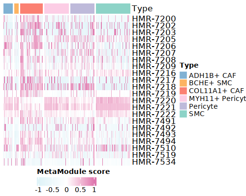
doheatmap_feature(Metacell.gsva,sample_info,top10$gene,9,9,cols=c('SMC'='#8DD3C7','MYH11+ Pericyte'='#FCCDE5','Pericyte'='#BEBADA','COL11A1+ CAF'='#FB8072','ADH1B+ CAF'='#80B1D3','BCHE+ SMC'='#FDB462'))

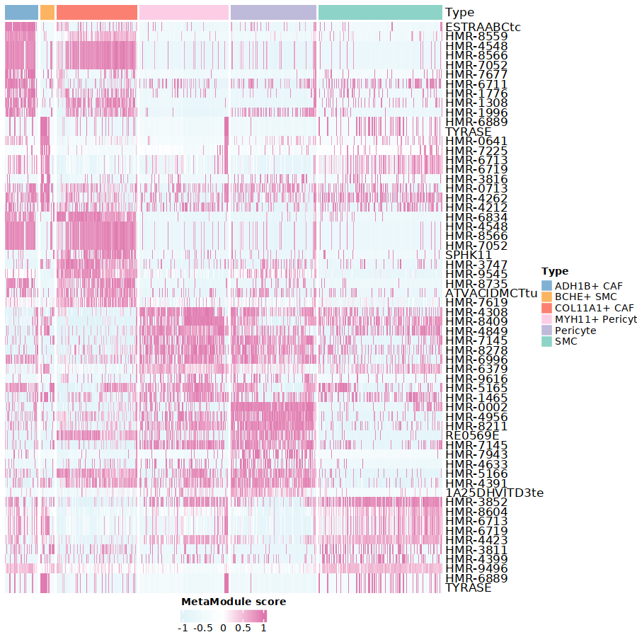
In our fibroblast integration data, we found that CTHRC1+ CAFs showed higher MetaModule scores for chondroitin sulfate biosynthesis (HMR_7493 and HMR_7494). In this dataset, COL11A1+ CAFs exhibited a similar pattern.

doheatmap_feature(Metacell.gsva.seurat,'cell_type',MM.meta[MM.meta$SUBSYSTEM=='Chondroitin / heparan sulfate biosynthesis','ID'],5,4, cols=c('SMC'='#8DD3C7','MYH11+ Pericyte'='#FCCDE5','Pericyte'='#BEBADA','COL11A1+ CAF'='#FB8072','ADH1B+ CAF'='#80B1D3','BCHE+ SMC'='#FDB462'))

Step 3 MetaRegulon analysis

MetroSCREEN systematically analyzes the combined effects of intrinsic cellular drivers and extrinsic environmental factors on metabolic regulation.

1. Prepare the essential files

Find the marker genes for each cell subtype, this is the basis for MetaRegulon activity calculation.

## Find the marker genes for each cell subtype of the Metacell object
Metacell.seurat<-readRDS('./scRNA/fibro_new_Metacell_seurat.rds')
Metacell.seurat.markers <- FindAllMarkers(Metacell.seurat, only.pos = TRUE)
Metacell.seurat.markers=Metacell.seurat.markers[Metacell.seurat.markers$p_val_adj<0.05,]
Metacell.seurat.markers=Metacell.seurat.markers[order(Metacell.seurat.markers$avg_log2FC,decreasing = TRUE),]
saveRDS(Metacell.seurat.markers,'./scRNA/fibro_new_Metacell_gene_markers.rds')

Prepare the Lisa results for each group, as these are essential for calculating MetaRegulon TR activity. Users can learn more about Lisa here.

for (i in unique(Metacell.seurat.markers$cluster)){
   df=Metacell.seurat.markers[Metacell.seurat.markers$cluster==i,]
   if (nrow(df)>500){
      genes=df[,'gene'][1:500]
   } else{
      genes=df[,'gene']
   }

   write.table(genes,paste0('./scRNA/lisa/',i,':marker.txt'),
         sep='\t',
         quote=F,
         row.names=FALSE,
         col.names=FALSE)
}

## Run this under Lisa's guidance
lisa multi hg38 ./scRNA/lisa/*.txt -b 501 -o ./scRNA/lisa/

2. Calculate the MetaRegulon score

The MetaRegulon for a MetaModule can be inferred using the cal_MetaRegulon function. MetroSCREEN employs a four-step strategy to deduce the MetaRegulon: Inferring the activity of the MetaRegulon is the first step.

Correlating MetaRegulon activity with gene expression within the MetaModule constitutes the second step. We consider the highest correlation value among the genes in a MetaModule as representative of the interaction between the MetaRegulon and the MetaModule.

Using a multi-objective optimization method to determine the most likely MetaRegulon to control the MetaModule is the third step.

Inferring causation between the MetaModule and MetaRegulon using a PC-based method is the fourth step.

## Users can replace the metabolic reaction with one they are interested in
MM=readRDS("./ref/MM.nodup.rds")
MM.meta=readRDS("./ref/MM.meta.rds") %>%
   as.data.frame()
rownames(MM.meta)=MM.meta$ID

MetaModule.markers<-readRDS('./scRNA/fibro_new_Metacell_gsva_markers.rds')
Metacell.seurat<-readRDS('./scRNA/fibro_new_Metacell_seurat.rds')
Metacell.seurat.markers<-readRDS('./scRNA/fibro_new_Metacell_gene_markers.rds')

## set the parameters
object=Metacell.seurat
feature='cell_type'
state='COL11A1+ CAF'
## Users can use the differentially enriched MetaModule
# interested_MM=MetaModule.markers[MetaModule.markers$cluster=='COL11A1+ CAF','gene']
interested_MM=c('HMR-7493','HMR-7494')
MM_list=MM
markers=Metacell.seurat.markers
lisa_file='./scRNA/lisa/COL11A1+ CAF:marker.txt.lisa.tsv'
ligand_target_matrix='./ref/ligand_target_matrix.rds'
lr_network='./ref/lr_network.rds'
sample_tech='scRNA'
output_path='./scRNA/'
RP_score='./ref/RP_score.rds'
file_name='COL11A1_CAF'

Calculate the MetaRegulon score

cal_MetaRegulon(object,feature,state,interested_MM,MM_list,markers,lisa_file,ligand_target_matrix,lr_network,sample_tech,output_path,RP_score,file_name)

The results of the cal_MetaRegulon function will be stored in the ./scRNA/COL11A1_CAF/ floder, and the detailed information is shown below.

File | Description
{file_name}.rds	The expression matrix of the state.
{file_name}:lr_activity.rds	The ligands activity for each Metacell.
{file_name}:tr_activity.rds	The transcriptional regulators activity for each Metacell.
{file_name}:gg_activity_cor.rds	The correlation of intrinsic signaling components activity with MetaModule.
{file_name}:tr_activity_cor.rds	The correlation of intrinsic transcriptional regulators activity with MetaModule.
{file_name}:lr_activity_cor.rds	The correlation of extrinsic ligands activity with MetaModule.
./MetaRegulon/{file_name}:*.txt	The MetaRegulon results.

3. Downstream analysis

Resources of the MetaRegulon.

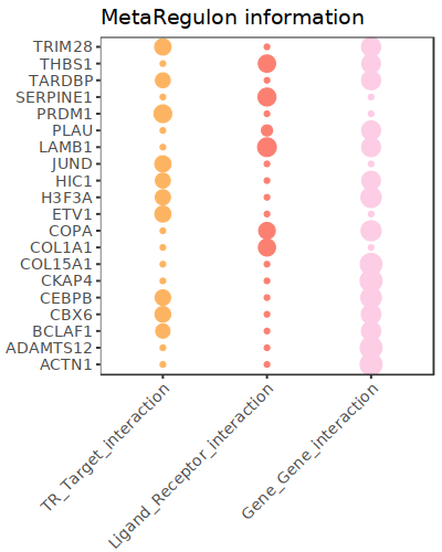
hmr_7494<-read.csv(paste0(output_path,file_name,'/MetaRegulon/',file_name,':HMR-7494.txt'),row.names = 1)
head(hmr_7494,2)
# TR_Target_interaction      Ligand_Receptor_interaction     Gene_Gene_interaction   ag_score        .level  Final_score     gene    rank    resource        direction
# <dbl>      <dbl>   <dbl>   <dbl>   <int>   <dbl>   <chr>   <int>   <chr>   <chr>
# CKAP4      0       0.000000        0.4888826       0.02205261      1       0.02205261      CKAP4   1       intrinsic       regulator
# LAMB1      0       0.312634        0.3241996       0.02205261      1       0.02205261      LAMB1   2       intrinsic       effector
df_use=melt(hmr_7494[1:20,c(1:3,7)])

width=4
height=5
options(repr.plot.width =width, repr.plot.height = height,repr.plot.res = 100)
ggplot(df_use, aes(x = variable, y = gene)) +
   geom_point(aes(color = variable, size = value)) +
   scale_color_manual(values = c("TR_Target_interaction" = "#FDB462", "Ligand_Receptor_interaction" = "#FB8072",'Gene_Gene_interaction'='#FCCDE5')) +
   theme_bw() +
   theme(
      panel.grid.major = element_blank(),
      panel.grid.minor = element_blank(),
      axis.text.x = element_text(angle = 45, hjust = 1),
      legend.position = "none"
   ) +
   theme(axis.title = element_text(size = 10), axis.text = element_text(size = 10),
         legend.text = element_text(size = 10), legend.title = element_text(size = 10))+
   labs(x = NULL, y = NULL, title = "MetaRegulon information")

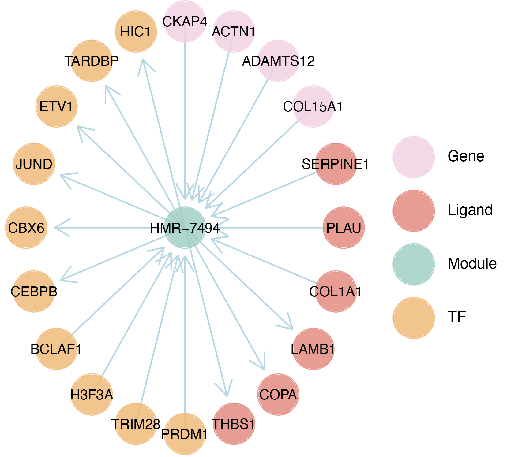
Build the network.

hmr_7494<-read.csv(paste0(output_path,file_name,'/MetaRegulon/',file_name,':HMR-7494.txt'),row.names = 1)
df_use=hmr_7494[1:20,]
network=data.frame(from=rownames(df_use),to='HMR-7494',label=ifelse(df_use$direction=='regulator','1','2'),
                  color=ifelse(df_use$gene %in% df_use[df_use$Ligand_Receptor_interaction>0,'gene'],'Ligand',
                              ifelse(df_use$gene %in% df_use[df_use$TR_Target_interaction>0,'gene'],'TF','Gene')))
network <- network %>%
   mutate(
      from_new = ifelse(label == 2, to, from),
      to_new = ifelse(label == 2, from, to)
   ) %>%
   select(from = from_new, to = to_new, label, color)
node=data.frame(unique(c(network$from,network$to)))
node$class=ifelse(node[,1] %in% 'HMR-7494','Module',
                  ifelse(node[,1] %in% df_use[df_use$Ligand_Receptor_interaction>0,'gene'],'Ligand',
                     ifelse(node[,1] %in% df_use[df_use$TR_Target_interaction>0,'gene'],'TF','Gene')))
colnames(node)=c('gene','class')
g <- graph_from_data_frame(d = network, vertices =node, directed = TRUE)
layout <- create_layout(g, layout = 'circle')

## Modify the layout
n=nrow(layout[layout$class %in% c('Ligand','TF'),c('x','y')])
theta <- seq(0,2*pi, length.out = 21)
coords <- data.frame(
x = sin(theta) ,
y =  cos(theta) )
layout[layout$class=='Gene',c('x','y')]=coords[1:4,]
layout[layout$class=='Ligand',c('x','y')]=coords[5:10,]
layout[layout$class=='TF',c('x','y')]=coords[11:20,]
layout[layout$class=='Module','x']=0
layout[layout$class=='Module','y']=0

Draw the network

width=5
height=5
options(repr.plot.width =width, repr.plot.height = height,repr.plot.res = 100)
output_name='HMR-7493.pdf'

graph_g<-ggraph(layout)+   #kk
   geom_edge_link(color='lightblue',arrow = arrow(length = unit(5, 'mm')),end_cap = circle(8, 'mm'))+
   geom_node_point(aes(color=class),size = 15,alpha=0.8)+
   geom_node_text(aes(label = name),size=4) +
   scale_color_manual(values = c('Ligand'="#FB8072",'TF'="#FDB462",'Gene'='#FCCDE5','Module'='#8DD3C7')) +
   scale_edge_width(range=c(0.5,1.5))+
   theme(text = element_text(size=8))+
   theme_void()
print(graph_g)
pdf(paste0(output_path,output_name),width=width,height=height)
   print(graph_g)
dev.off()